Welcome to Taxo Tape
How to Model Thermal Resistance in TIM Layers – A Practical Guide for Engineers
Introduction
Accurate thermal modeling has become a critical step in power electronics and electronic system design. As devices become smaller and more powerful, the heat generated by semiconductors, MOSFETs, and IGBTs must be efficiently transferred to heatsinks or chassis. Without proper thermal control, even a small rise in junction temperature can significantly shorten component life or cause performance drift.
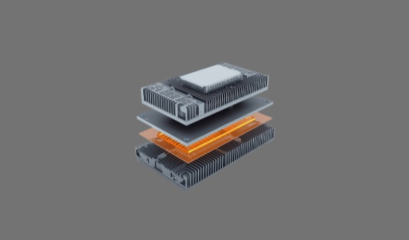
In this context, Thermal Interface Materials (TIMs) play a vital role. They fill microscopic air gaps between mating surfaces—such as between a power device and a heatsink—creating a more effective thermal path. Selecting the right TIM and correctly modeling its thermal resistance ensures that simulations match real-world performance, enabling engineers to design reliable systems with predictable temperature profiles.
However, engineers often make three common mistakes when estimating TIM behavior:
Treating the TIM as a uniform, ideal thermal layer and ignoring contact resistance.
Assuming thermal conductivity values from datasheets without considering compression or interface quality.
Underestimating the influence of bond line thickness (BLT) and surface flatness on actual heat transfer.
This article provides a practical framework for modeling thermal resistance in TIM layers, helping engineers bridge the gap between theoretical design and real-world thermal performance.
Understanding Thermal Resistance in TIMs
Definition and Basic Equation
Thermal resistance () quantifies how efficiently heat flows through a material. It is defined as:
where:
= thermal resistance (K/W)
= material thickness (m)
= thermal conductivity (W/m·K)
= effective contact area (m²)
In essence, the thinner the layer and the higher the thermal conductivity, the lower the resistance. For a given material, reducing thickness or increasing the contact area directly enhances heat transfer efficiency. However, this simplified equation assumes a perfect interface, which is rarely achievable in real applications.
Bulk Resistance vs. Contact Resistance
In practical assemblies, total thermal resistance is the sum of bulk resistance and contact resistance:
While bulk resistance depends on the intrinsic conductivity and thickness of the material, contact resistance arises from microscopic surface roughness, air gaps, and insufficient wetting between the two surfaces.
Even highly conductive TIMs can underperform if interface pressure is too low or if the surfaces are uneven. In fact, in many electronic assemblies, contact resistance dominates total thermal resistance—sometimes accounting for more than 60% of the overall temperature drop across the interface.
Modeling Thermal Resistance Step-by-Step
Step 1 – Identify Material Properties
The accuracy of any thermal model depends on using realistic material parameters. The most critical ones are thermal conductivity (k) and compressibility.
Thermal conductivity determines how efficiently heat moves through the material, while compressibility defines how much the TIM deforms under pressure to conform to the mating surfaces.
Material formulation strongly affects these values:
Filler type (e.g., alumina, boron nitride, or graphite) influences both conductivity and viscosity.
Filler loading affects the percolation path for heat flow.
Binder system (silicone, acrylic, or epoxy) determines long-term mechanical stability.
For accurate modeling, use measured data under similar conditions to the intended application—especially temperature, compression, and aging state.
Step 2 – Define Bond Line Thickness (BLT)
The bond line thickness is one of the most influential parameters in TIM performance. BLT depends on the amount of applied material, surface flatness, and clamping pressure during assembly.
Higher pressure generally reduces BLT, improving thermal conduction—up to a point. If the layer becomes too thin, the TIM may fail to accommodate surface roughness, leading to incomplete contact or even electrical shorting (in the case of conductive fillers).
To estimate or measure BLT:
Use mechanical stack-up simulations or direct displacement sensors in test fixtures.
Refer to manufacturer data that correlates pressure and thickness.
Thinner is not always better. The optimal BLT minimizes both bulk and contact resistance without compromising electrical insulation or mechanical integrity.
Step 3 – Calculate Effective Thermal Resistance
Once you have , , and , start with the bulk resistance:
Then, add the contact resistance term, derived from empirical data or measurement:
Example:
For a silicone-based TIM with , , and , the bulk resistance is:
If contact resistance adds 0.005 K/W under typical assembly pressure, the total is .
Simulation results should be validated against measured thermal impedance to ensure the model represents actual interface conditions.
Step 4 – Validate with Experimental Testing
Modeling alone cannot capture every real-world variable. Therefore, validation using standardized testing methods is essential.
Common approaches include:
ASTM D5470: The industry-standard steady-state test for measuring thermal resistance under controlled pressure and temperature.
Transient methods: Such as laser flash or transient plane source, for rapid evaluation of thermal impedance.
When interpreting test data, consider both the slope (indicating bulk conductivity) and the intercept (representing contact resistance).
Finally, use this data to calibrate your simulation models, adjusting for real contact behavior, compression, and interface roughness. This ensures that your thermal simulations accurately predict system-level performance before prototypes are built.
Factors Affecting Thermal Resistance Accuracy
Surface Flatness and Pressure
The physical condition of mating surfaces has a direct impact on the actual thermal contact achieved by a TIM layer. Uneven or warped surfaces create microscopic air gaps that act as thermal insulators, leading to localized hotspots and inconsistent heat spreading.
Applying the correct compression force is essential to minimize these gaps. Under sufficient pressure, the TIM deforms and fills surface irregularities, lowering contact resistance. However, excessive compression can squeeze out material or damage components, while too little pressure leaves voids.
When modeling, engineers should include pressure-dependent contact resistance or use data obtained under representative clamping forces to ensure the model reflects real assembly conditions.
Temperature and Aging Effects
Thermal and mechanical properties of TIMs evolve with time and temperature exposure. During prolonged operation or thermal cycling, filler-matrix interfaces may degrade, and the material may soften, harden, or separate.
For example:
Silicone-based greases may experience pump-out or oil bleeding.
Phase-change materials can show slight conductivity drift after thousands of cycles.
Elastomer pads may lose elasticity, increasing BLT and contact resistance.
To improve model reliability, it is important to integrate temperature-dependent material data and, if possible, aging correction factors derived from accelerated life testing. This allows engineers to predict long-term thermal resistance growth and make lifetime reliability assessments early in the design process.
Interface Voids and Assembly Quality
Voids and trapped air are among the most common—and most harmful—defects in thermal interfaces. They can result from poor dispensing control, trapped contamination, or uneven surface pressure, and can drastically increase local resistance.
A single 5% void fraction can raise the total interface resistance by more than 20%, depending on the TIM type. Voids also create temperature gradients that accelerate material aging and reduce system reliability.
During modeling, engineers can simulate the effect of voids by reducing effective contact area (A) or introducing an air-gap layer with low conductivity (~0.026 W/m·K). This helps visualize how assembly quality affects the overall heat path and guides improvements in process design.
Practical Modeling Tools and Simulation Tips
Several powerful software tools can be used to model TIM performance:
ANSYS Fluent / Icepak – for detailed steady-state and transient heat transfer analysis.
COMSOL Multiphysics – for parametric studies involving coupled thermal-mechanical behavior.
Siemens Simcenter – for full-system thermal simulations with contact modeling capabilities.
For early design stages, simplified equivalent thermal circuits can be used to estimate junction-to-ambient performance quickly. By representing each layer as a resistor, engineers can easily compare different stack-up configurations before building detailed 3D models.
Tips for improving model accuracy:
Use measured material data instead of generic datasheet values.
Include surface roughness and contact pressure as boundary parameters.
Validate models with at least one physical measurement (e.g., ASTM D5470 test).
Optimize mesh density only around thermal interfaces to reduce computation time.
Combining these techniques ensures that modeling is both efficient and representative of real-world performance.
Case Example: Comparing Different TIM Types
To illustrate how modeling supports design decisions, consider three common TIM categories: silicone grease, phase-change materials (PCM), and thermal pads.
| TIM Type | Typical Conductivity (W/m·K) | Model Behavior | Reliability Trend |
|---|---|---|---|
| Thermal Grease | 2–5 | High initial performance; sensitive to pump-out | Moderate; requires maintenance |
| Phase-Change Material | 2–6 | Stable under cycling; low contact resistance | Excellent long-term stability |
| Thermal Pad | 1–3 | Simple to apply; constant BLT | Good; limited for high-power density |
By modeling each option under identical conditions, engineers can predict junction temperature differences before prototype testing. This reduces design iteration cycles and helps select the most suitable TIM early, improving cost and reliability outcomes.
Conclusion
Accurate modeling of thermal resistance in TIM layers is essential for reliable heat management in modern electronics. Surface flatness, applied pressure, material degradation, and assembly quality all significantly influence the final thermal path.
By combining precise material data, validated test results, and realistic boundary conditions, engineers can create predictive models that align closely with experimental outcomes.
Integrating these insights early in the design stage leads to better component selection, fewer failures, and optimized thermal performance across the system’s lifetime. In short, a well-modeled TIM interface is the foundation of a reliable thermal design.